Browse & Filter

Let
$$\frac{\partial (x,y)}{\partial (a,b)}\,\equiv\,\left|\begin{array}{ll}
\frac{\partial x}{\partial a}&\frac{\partial y}{\partial a}\\
\frac{\partial x}{\partial b}&\frac{\partial y}{\partial b}\\
\end{array}\right|$$

Then show that
$$ \frac{\partial (x,y)}{\partial (a,b)}\frac{\partial (a,b)}{\partial (c,d)}\,=\,\frac{\partial (x,y)}{\partial (c,d)} $$

Remarks : 1. This can be generalised to higher dimensions.

2. This can be found in books - and is very useful in changing variables in multiple integrals.

The equation of continuity for conservation of electric is derived. An expression for current in a wire is obtained in terms of number of electrons per unit volume.

A system consists of three particles and each particle can exist in five possible states. Find the total number of microstates and the number of microstates that energy level has two particles assuming

• the particles are non-identical
• are identical bosons
• are identical fermions.

Electrodynamics                                                           Feb 27, 2019
                              MID SEMESTER EXAMINATION — Extra Set

1. A gold nucleus contains a positive charge equal to that of 79 protons. An$\alpha$ particle, $Z=2$, has kinetic energy $K$ at points far away from thenucleus and is traveling directly towards the charge, the particle just touchesthe surface of the charge and is reversed in direction. relate $K$ to the radiusof the gold nucleus. Find the numerical value of kinetic energy in MeV is theradius $R$ is given to be $5 \times10^{-15}$ m. \centerline {[ 1 MeV = $10^6$eV and 1 eV = $1.6\times10^{-16}$]

2. A line charge carrying a charge \(\lambda\) per unit length and extending from \((-a,0,0)\) to \((+a,0,0)\) lies along the \(x\)- axis. Find the potential at a point on the \(X\)- axis at point \((x,0,0), x>a\) and at a point \((0,y,0)\) on the \(Y\)-axis. Complete the integrations as much as you can.
3. Two infinitely conducting coaxial cylinders have radii $a,b$ respectively.
   1. Compute the electric field between the cylinders.
   2. Find the electrostatic energy per unit length of the capacitor formed by the cylinders by integrating expression for the energy stored per unit volume of the electric field.
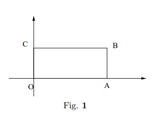
4. Solve Laplace equation inside a rectangle \(OABC\) with corners at \((0,0), (a,0), (a,b),(0,b)\) respectively. The sides \(OA\) and \(OB\) are held at zero potential and the sides \(AB\) and \(BC\) are kept at constant potential \(V_0\)

In this lecture canonical ensemble and canonical partition function are introduced. This topic has a central place in equilibrium statistical mechanics. This ensemble describes the microstates of a system in equilibrium with a heat bath at temperature T . The probability of a microstate having energy E is proportional to $exp(−βE)$ where $ β = kT $ and k is Boltzmann constant.

$\newcommand{\DD}[2][]{\frac{d^2 #1}{d^2 #2}}$ 
$\newcommand{\matrixelement}[3]{\langle#1|#2|#3\rangle}$
$\newcommand{\PP}[2][]{\frac{\partial^2 #1}{\partial #2^2}}$
$\newcommand{\dd}[2][]{\frac{d#1}{d#2}}$
$\newcommand{\pp}[2][]{\frac{\partial #1}{\partial #2}}$
$\newcommand{\average}[2]{\langle#1|#2|#1\rangle}$