[NOTES/QM-13004] General Properties of Motion in One Dimension

1. Bound state eigenvalues are non-degenerate :

Proof:
We shall show that if for a given bound state energy eigenvalue $E$ there are two eigenfunctions $\psi_1$ and $\psi_2$, the two solutions must be proportional. Thus we have \ref{eq101} and \eqref{eq102} \begin{eqnarray} -\frac{\hbar^2}{2m}\frac{d^2\psi_1}{dx^2} + V \psi_1 &=& E\psi_1 \label{eq101}\\ -\frac{\hbar^2}{2m}\frac{d^2\psi_2}{dx^2} + V\psi_2 &=& E\psi_2 \label{eq102} \end{eqnarray} Multiply \eqref{eq101} by $\psi_2$ and \eqref{eq102} by $\psi_1$ and subtract to get \begin{eqnarray} -\frac{\hbar^2}{2m} \left(\psi_2\frac{d^2\psi_1}{dx^2} - \psi_1\frac{d^2\psi_2}{dx^2}\right) &=& 0\\ \mbox{or}\qquad\qquad {d\over dx} \left(\psi_2{d\psi_1\over dx} - \psi_1{d\psi_2\over dx}\right) &=& 0 \end{eqnarray} Integrating we get $$ \left(\psi_2{d\psi_1\over dx} - \psi_1{d\psi_2\over dx}\right) = \mbox{const.}~,C $$ The constant $C$ can be fixed by evaluating the left hand side at $x=\infty$. As $x\to\pm\infty$, $\psi_1\to0$, $\psi_2\to0$ for bound states\\ $\therefore~~~C=0$\\ Thus we get \begin{eqnarray} \psi_2{d\psi_1\over dx} - \psi_1{d\psi_2\over dx}&=& 0\\ \mbox{or}\qquad\qquad {1\over \psi_1} {d\psi_1\over dx} - {1\over\psi_2}{d\psi_2\over dx} &=& 0 \end{eqnarray} Integrating we get \begin{eqnarray} \ln \psi_1 - \ln\psi_2 &=& \mbox{const.,}~~K\\ \mbox{or}\qquad\qquad \ln(\psi_2/\psi_1)&=& \ln K\\ \mbox{or}\qquad\qquad \psi_2 &=& K\psi_1 \end{eqnarray} $\therefore ~\psi_1$ and $\psi_2$ are linearly dependent. Hence the bound state eigenvalues in one dimension are {\it non degenerate}. An exception to this result is particle in twin, (or more) boxes described by the potential .

$ V(x) = \begin{cases}0 & \mbox{$ 0\le x \le L $}\cr 0 & \mbox{$ 2L\le x \le 3L$ }\cr \mbox{$ \infty $} & \mbox{ otherwise } \end{cases} $ .

For this potential each energy eigenvalue has two linearly independent solutions.

2. Behaviour of the energy eigenfunctions for large distances:

Consider the motion of a particle in one dimension in a potential $V(x)$ such that

• [a) $V(x)$ has a minimum value $V_{\mbox{min}}$
• [b) as $x\to +\infty$~~ $V(x)\to V_+$
• [c) as $x\to -\infty$~~ $V(x)\to V_-$

Then the large distance behaviour of the corresponding energy eigenfunction is as follows.

• [a) The energy eigenfunction for $E$ less than both \(V_\pm\) is exponentially damped

  \begin{eqnarray}\psi_E(x) \longrightarrow\exp(-\alpha_1 x) & \mbox{ as } \qquad x\to\infty \psi_E(x)\longrightarrow\exp(\alpha_2 x)~ & \mbox{ as }\qquad x\to-\infty \end{eqnarray}

  where= $\alpha_1=\sqrt{\frac{2m(V_+-E)}{\hbar^2}}, ~~\alpha_2=\sqrt{\frac{2m(V_- -e)}{\hbar^2}}$
• (b) For $E$ gretear than both \(V_\pm\) , the solution behaves like plane waves (i.e., it is oscillatory) at large distances. As $x \to \infty $ \begin{eqnarray} \psi(x) \to \begin{cases}A\cos k_1x + B\sin k_1 x &\cr \mbox{or} &\cr Ae^{ik_1x} + Be^{-ik_1x} & ~~~ k_1 =\sqrt{2m(E-V_+)}{\hbar^2} \end{cases} \end{eqnarray} and as $x \to -\infty$ we get $$ \psi(x) \to \begin{cases}A\cos k_2x + B\sin k_2 x \cr \mbox{or} &\cr Ae^{ik_2x} + Be^{-ik_2x} & ~~~ k_2 =\ \frac{\sqrt{2m(E-V_-)}}{\hbar^2} \end{cases} $$

The above results can be seen easily  by replacing the potential by its limiting value \(V_+\) or \(V_-\), and 
solving the resulting  differential equation.

3.Nature and degeneracy of energy eigenvalues:

The nature of energy eigenvalues, discrete or continuous, degenerate or non-degenerate, is generally given by the following rules. It may be added that the rules give us an idea what to expect for given potential and that exceptions to some of these rules below are known to exist.

• It can be proved that the energy eigenvalues must be greater than or equal to $V_{\mbox{min}}$.
• Bound states exist for energy greater than $V_{\mbox{min}}$ and but below both $V_+$ and $V_-$. The corresponding energy eigenvalues are discrete and nondegenerate.
• For $E$ between $V_+, V_-$, the eigenvalues are continuous and non-degenerate.
• For $E$ greater than both $V_+$ and $V_-$, the energies are continuous and doubly degenerate.

You may check validity of these rules for the potential problems for which you have seen exact solutions such as square well, harmonic oscillator and other potentials .

4.Minimum bound state energy:

If the potential function has a minimum at $x_o$ with a value $V_{\mbox{min}}$. In classical mechanics, a state with zero momentum, $p=0$, and $x=x_o$ can exist and the energy will be $V_{\mbox{min}}$. In QM $x$ and $p$ cannot have sharp values simultaneously, and for the lowest bound state the energy will, in general, be greater than $V_{\mbox{min}}$. The ground state energy can be estimated using the uncertainty principle. We shall illustrate this by means of the harmonic oscillator. $$ V(x) = {1\over2} m\omega^2 x^2 $$ $V_{min}=0$ classically $x=0$, $p=0$, $E=0$ is a possible state. Quantum mechanically, the values of $x$ and $p$ will have some uncertainties $\Delta x$ and $\Delta p$ which are subject to the uncertainty relation~~ $\Delta p \Delta x \simeq \hbar$. Taking the averages of $x^2$ and $p^2$ of the order of $(\Delta x )^2$ and $(\Delta p)^2 $, respectively, and using $\Delta p \approx \frac{\hbar}{\Delta x}$, we have \begin{eqnarray} < KE >~ & \approx& {(\Delta p)^2\over2m} = \frac{\hbar^2}{2m(\Delta x)^2}\\ <v(x)>&\approx& {1\over2} m \omega^2(\Delta x)^2\\ E &\approx& {\hbar^2\over2m}\left({1\over\Delta x}\right)^2 + {1\over2} m\omega^2(\Delta x)^2 \end{eqnarray} Minimizing $E$ w.r.t. $\Delta x$ we get \begin{eqnarray} {\hbar^2\over2m}\left({-2\over(\Delta x)^3}\right) + {1\over2} m\omega^2 2(\Delta x) &=& 0\\ (\Delta x)^4 &=& {\hbar^2\over2m} \times {2m\over m\omega^2}\\ (\Delta x)^2 &=& {\hbar\over m\omega}\\ E&\approx& {\hbar^2\over2m} {m\omega\over\hbar} + {1\over2} m\omega^2{\hbar^2\over m\omega}\\ &=& \hbar\omega \end{eqnarray} If we had used $\Delta p \Delta x \ge \hbar/2$ we would have obtained $$ E_{min} = {\hbar\omega\over 2} $$ which matches with the exact ground state energy of the harmonic oscillator. In general this argent can be used to get a quick estimate of the ground state energy for a given potential.

5.Parity

If the potential is an even function of $x$,{\it i.e.}, $V(-x)=V(x)$, the parity operator commutes with the Hamiltonian. \begin{equation} \hat{P} \hat{H} - \hat{H} \hat{P} =0 \end{equation} If $u_E(x)$ is an eigenfunction of energy with eigenvalue $E$, $v(x)=Pu(x)=u(-x)$ is also an eigenfunction of Hamiltonian with the same eigenvalue $E$. This is easily seen by applying $\hat{H}$ on $v(x)$. \begin{eqnarray} \hat{H} v(x) &=& \hat{H}\hat{P}u(x)\\ &=& \hat{P}\hat{H}u(x)\\ &=& E \hat{P} u(x)\\ &=& E v(x) \end{eqnarray} Now there are two possibilities.

1. When the eigenvalue is non-degenerate there is only one linearly independent eigenfunction and $u(x)$ and $v(x)$ must be proportional. There must exist a constant $c$ such that \begin{equation} u(x) = c v(x) \label{tmp1} \end{equation} Noting the relation $v(x)=u(-x)$, we have \begin{equation} u(x) =c u(-x) \label{tmp2} \end{equation} Making a replacement $x \to -x$ in this equation implies \begin{equation} u(-x)=cu(x) \end{equation} Now \eqref{tmp1} and \eqref{tmp2} imply that $c^2=1$ and hence $c=\pm1$. This gives $u(x)=\pm u(-x)$ and $u(x)$ must be an eigenfunction of parity.
2. In the second case when $u(x)$ and $v(x)$ are linearly independent, $v(x)$ is a new solution of the eigenvalue problem. This happens if and only if the energy is degenerate. This is the case for example for a symmetric square well for positive energies. If form the combinations $w_1(x), w_2(x)$ defined by \begin{eqnarray} w_1(x) &=& u(x) + v(x) = u(x) + u(-x)\\ w_2(x) &=& u(x) - v(x) = u(x) -u(-x) \end{eqnarray} and these will be eigenfunctions of parity. Similar comments, though differing in details, will apply for any operator which commutes with Hamiltonian of the system.

6.Tunnelling through a barrier

Consider an example of a particle initially confined to a box whose walls can be represented by a potential barrier of finite height $V_0$. For example, considering a one dimensional box having walls represented by a potential of height $V_0$. Let the potential inside the box be zero. If the energy of the particle is less than barrier height $V_0$, classically the particle will always remain confined to the box.

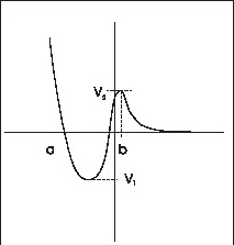
Similarly, for the two potentials shown in Fig. 1 the bounded motion is possible for a classical particle for energies between $V_1$ and $V_2$.  if the particle is on the left of the maximum at $x=b$, it cannot cross the barrier at x=b when $E < V_2$. However, in quantum mechanics for the potential in Fig. 1  there is no bound state in the range $V_1 < E < V_2$ . For potential of Fig. 1 there are no bound states at all.

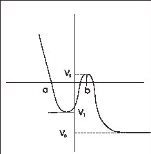
For the potential of Fig.2, the  bound states energy must lie between $0$ and $V_1$,  There is no bound state for \)E>0\) This happens because quantum mechanically a particle can cross a barrier even if it has energy less than the barrier height. Exactly in a similar fashion, a classical particle incident from the right ($ x> b$) with $E< 0$ cannot reach the region $x<b$, whereas a quantum particle can. This phenomenon is known as barrier penetration or tunnelling. earliest know example of tunnelling phenomenon is $\alpha $ decay.

Fig 1  For potential in this figure there is no quantum bound state for \(V_1<E< V_2\). Compare this with classical case, when bounded motion is possible.	Fig 2 In the potential in this figure there will be bound states for energy between 0 and \(V_1\)

Important: It must emphasized that the tunnelling across a barrier takes place, only if after tunnelling the potential energy is less than the energy and the classical motion is possible.

7.Periodic potentials, Energy bands

Let $V(x)$ be a periodic potential with period $L$ $$V(x+L) = V(x)\,\,\,.$$ The energy eigenvalues has bands of allowed energies and forbidden energies and the energy level diagram is schematically shown in Fig. 3

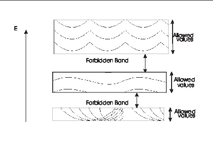Fig 3  Sketch of energy Bands in periodic potential