[NOTES/QM-13001] Square Well Energy Eigenvalues and Eigenfunctions

We shall discuss the energy spectrum for a square well potential shown in figure below. Within the range of the well, it is an attractive, and constant, potential. With suitable reference for potential energy, the potential can be chosen to be $0$ inside the well. It is again a constant outside the range of the potential well. We have chosen $V_0 > 0$ to denote the value of the potential outside the well.

We shall now obtain the solution for energy levels of a square well potential in one dimension. 

Fig 1 Square  Well
\( V(x) = \begin{cases} 0, & 0< x<L\\ V_0 & \text{otherwise} \end{cases}\)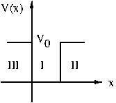

Since the potential has different expressions for different values of $x$, the Schr\"odinger equation is solved in the three regions (i) $x<0$, (ii) $0\le x\le L$, and (iii) $x>L$ separately. Also the two ranges of energy $0<E<V_0$ and $E>V_0$ will be considered separately.

Bound states

The bound states correspond to $0<E<V_0$. For the bound states one must insist that $\psi(x)\to 0$ at large distances, because $|\psi|^2dx$ represents probability of particle being found between $x$ and $x+dx$. Thus in the limit $x\to\pm\infty$, we must have $\lim \psi(x)\to 0$. The solutions will be obtained in the three regions I,II, and III separately. Besides vanishing of the solution at infinity, we shall impose the requirement of continuity on the solution for the eigenfunctions and their derivatives.

Region I, \(0\le x\le L :\)

The Schr\"odinger equation is
$$ -\frac{\hbar^2}{2m} \frac{d^2\psi}{dx^2} = E\psi $$
or
$$ \frac{d^2\psi}{dx^2} + k^2 \psi =0 $$
where $k^2=2mE/\hbar^2$ and most general solution is
$$ \psi_\text{I}(x) = A \sin kx + B \cos kx $$

Region II, \(x > L\) 

When $x>L$, $V(x)=V_0$ and the Schr\"odinger equation takes the form
$$ -\DD[\psi]{x} \frac{d^2\psi}{dx^2} + (V_0-E) \psi =0 $$
or
$$\frac{d^2\psi}{dx^2} + \frac{2m}{\hbar^2} (V_0-E) \psi =0$$
Noting \((V_0-E)> 0\), we use the notation $\frac{2m}{\hbar^2}(V_0-E)\equiv\alpha^2$, where $\alpha$ is real. The most general solution for $x<0$ is
$$ \psi_\text{II} = Ce^{\alpha x} + D e^{-\alpha x} $

 Region III, \(x>0\)

The solution for $x < 0$ , will have the same form as in the region II.
$$ \psi_\text{III} = F e^{\alpha x} + G e^{-\alpha x} $$

Boundary conditions at infinity

For the bound states the wave function must vanish for large distances.

• [(i)] We want that $\psi_\text{III}(x)$ should $\to 0 ~ \mbox{ as }~ x\to -\infty .$\\ $\therefore G=0$
• [(ii)]Also $\psi_\text{II}(x)$ should $\to 0$~~ as ~~ $x\to\infty$\\ $\therefore ~~ C=0$

 Continuity Conditions

Next we require that the wave function and its derivative be continuous at $x=0$ and $x=L$. Continuity conditions for the solution and its derivative at $x=0$ give
\begin{eqnarray} \psi_\text{III}(x)|_{x=0}&=&\psi_\text{I}(x)|_{x=0}\\ \psi^\prime_\text{III}(x)|_{x=0}&=&\psi_\text{I}^\prime(x)|_{x=0} \end{eqnarray}
writing out these and using $G=0$ gives
\begin{eqnarray} F &=& B \\ \alpha F &=& kA \end{eqnarray}
which implies
\begin{equation}
B =k A \alpha \label{EQ16}
\end{equation}

Continuity conditions for the derivative at $x=L$ give
\begin{eqnarray} \psi_\text{I}(x)|_{x=L}&=&\psi_\text{II}(x)|_{x=L}\\ \psi^\prime_\text{I}(x)|_{x=L}&=&\psi_\text{II}^\prime(x)|_{x=L} \end{eqnarray}
These equations imply
\begin{eqnarray} A \sin kL + B \cos kL &=& D e^{-\alpha L} \label{EQ4A}\\ kA \cos kL - k B \sin kL &=& -D \alpha e^{-\alpha L}\label{EQ4D} \end{eqnarray}

Bound State Energies

We use \eqref{EQ16} to eliminate $B$ in favour of $A$, next using \eqref{EQ4A} and \Ref{EQ4D} we get two equations for $A$ and $D$. These two equations can be written in form of a matrix
$$ \left[\begin{array}{cc} \sin kL + \frac{k}{\alpha} \cos kL & - e^{-\alpha L}\\ k\cos kL -\frac{k^2}{\alpha} \sin kL & \alpha e^{-\alpha L} \end{array}\right]~ \left[\begin{array}{c} A\\ D \end{array}\right] = 0 $$

These equations have a non trivial solution only when the determinant of the matrix on left hand side is zero. This requirement gives a condition on the allowed values of energy and can be cast in the forms \begin{eqnarray} \alpha ( \sin kL + \frac{k}{\alpha} \cos kL ) + ( k\cos kL -\frac{k^2}{\alpha} \sin kL ) &=&0 \\ (k^2 - \alpha^2 ) \sin kL - 2k\alpha \cos kL &=&0. \end{eqnarray}
{\it i.e.}
\begin{equation} \tan kL = \frac{2k\alpha}{k^2-\alpha^2} \equiv \tan2\theta, \end{equation}
where $\theta$ is defined by $\tan\theta = \alpha/k$, it is now easy to see that bound state energy eigenvalue must satisfy, (Why?)
\begin{equation} k \tan kL/2 =\alpha, ~~~~~~~~\mbox{\rm or} ~~~~~~~~~~~~~ k \cot kL/2 = -\alpha \end{equation}
Energy $E$ appears in the above quantization condition through $k$ and $\alpha$. Possible values of energy can be determined graphically.