


 ||Message]
$\newcommand{\DD}[2][]{\frac{d^2 #1}{d^2 #2}}$
$\newcommand{\matrixelement}[3]{\langle#1|#2|#3\rangle}$
$\newcommand{\PP}[2][]{\frac{\partial^2 #1}{\partial #2^2}}$
$\newcommand{\dd}[2][]{\frac{d#1}{d#2}}$
$\newcommand{\pp}[2][]{\frac{\partial #1}{\partial #2}}$
$\newcommand{\average}[2]{\langle#1|#2|#1\rangle}$
qm-lec-16007
The potential for a rigid spherical box can be written as
\begin{equation} V(r) = \begin{cases} 0 ,& 0 < r < a\\ \infty, & r >a
\end{cases} \label{eq01}. \end{equation}
The problem is separable in spherical polar coordinates and form of the full
wave function is
\begin{equation} \psi(r,\theta, \phi) = R(r) Y_{\ell m}(\theta, \phi)
\label{eq02}. \end{equation}
We need to consider solutions of the radial equation only. No solution can be
found for $E< 0$, therefore we consider $E>0$. For $r>a$ the potential is
infinite and hence the radial wave function must be zero, Next we consider $r< a$, where the potential is zero. The radial equation assumes the form
\begin{equation} -\frac{1}{r^2}\dd{r} r^2 \dd[R(r)]{r} +
\frac{\ell(\ell+1)\hbar^2}{2mr^2} R(r) - E R(r) =0. \label{eq03} \end{equation}
The most general solution of this equation is given in terms of spherical
Bessel functions $j_\ell, n_\ell$ and we write it as
\begin{equation} R_{E\ell(r)} = A j_\ell(kr) + Bn_\ell(kr), \qquad k^2 =
\frac{2mE}{\hbar^2} \label{eq04}. \end{equation}
Recall that near $r=0$, $n_\ell(r) \sim r^{-\ell-1}$ and blows up as $r\to 0$.
Therefore we must set $B=0$ if the solution is to remain finite at $r=0$. Thus
we get
\begin{equation} R_\ell(r) = \begin{cases} A j_\ell(kr), & 0<r < a\\ 0 & r > a
\end{cases}.\label{eq05} \end{equation}
Next we must demand that the radial wave function $R(r)$ must be continuous at
$r=a.$ Remember that there is no corresponding requirement on the derivative
for this case of infinite jump in the potential at $r=a$ The continuity
requirement of $R_{E\ell}(r)$ becomes
\begin{equation} j_\ell(ka) = 0. \label{eq06} \end{equation}
The solutions of the above equation determine allowed values of $k$ and hence
allowed bound state energies.
Energy levels and degeneracy
To get all the solutions, one proceeds as follows. First set $\ell=0$ and
locate the roots of $j_0(ka)=0$. We call the roots as $\rho_{0n},
n=0,1,2,\ldots$ and the corresponding energies are given by
$E=\dfrac{\hbar^2\rho_{0n}^2}{2ma^2}$.. Here $n$ denotes the number of nodes of
the radial wave function for $\ell=0$.
Next, we set $\ell=1$ and find the roots
of $j_1(kr)=0$, calling these roots as $\rho_{1n}, n=0,1,2,\ldots$ the $\ell=1$
energy levels are given by $E=\frac{\hbar^2\rho_{1n}^2}{2ma^2}$. This process is
to be repeated for all values of angular momentum $\ell$ and the number of bound
states for each $\ell$ turns out to be infinite. The states of definite energy
depend on quantum numbers $n\ell m$ and the energy does not depend on magnetic
quantum number $m$. Therefore for a given azimuthal quantum number $\ell$ we
have $(2\ell+1)$ wave functions $N_{n\ell} R_{n\ell}(r/\rho_{n\ell})Y_{\ell
m}(\theta,\phi), (m=-\ell, -\ell+1,\cdots, \ell)$ and the energy levels
$E_{n\ell}$ are $(2\ell+1)$ fold degenerate. The energy increases with $\ell$
and also with increasing $n$. Thus schematic energy level diagram would appear
as follows.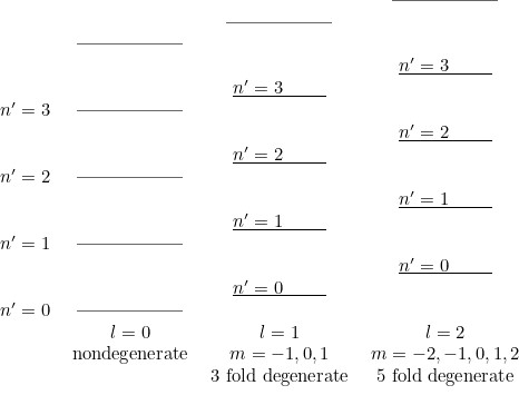
Exclude node summary :
Exclude node links:
4727: Diamond Point, 4909: QM-HOME-I
