[NOTES/CM-03001] Defining Action Functional

Configuration space
Let us consider a system with $N$ degrees of freedom. At a given time \(t\) the system is completely  specified by giving values the values of $N$ generalised coordinates \( q_1(t),\dots,q_N(t)\) and their time derivatives. We may arrange $q's$ in a row to form an $N$ component vector \begin{equation} \qbf = (q_1,q_2,\dots,q_N) \end{equation} the $N$ component vector can be represented by points in an $N$ dimensional space called configuration space. Conversely a point in {\it configuration space} represents a possible set of values of $(q_1,\dots,q_N)$

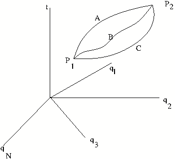
Paths in configuration space
With time $\qbf$ change and so also does the position of the point representing the system. Thus with time, the point representing the system will trace out a path in configuration space. This path in configuration space is obtained by solving the Euler Lagrange equations of motion. As Euler Lagrange equations are second order differential equations, the motion of the system, {\it i.e.} the state at any time, is completely known if we specify the initial values of $\qbf$ and $\dot \qbf$ at some time $t_0.$. With this as input, solving the Euler Lagrange equations of motion gives the generalised coordinates $\qbf(t)$ at all times, hence the path followed by system, in the configuration space is known.

Specifying coordinates at the end points
To solve the Euler Lagrange equations for  time \(t\) in the interval \((t_1,t_2)\), one may give boundary conditions on \(\qbf\) instead of initial conditions on \(\qbf, \dot\qbf\) at time \(t_1\). This means that coordinates $\qbf$ at the initial time $t_1$ and the final $t_2$ are to be specified. Thus we  look for solution of Euler Lagrange equations. \begin{equation} \qbf (t) = \{q_1(t),\dots,q_N(t)\}\quad \text{for} \quad  t_1\leq t\leq t_2 \end{equation} subjected to conditions \begin{equation} \qbf(t_1) = \{q_1(t_1),\dots,q_N(t_1)\}, \qquad \qbf(t_2) = \{q_1(t_2),\dots,q_N(t_2)\}. \end{equation} This amounts to asking what path is followed in configuration space, if we know the end points $P_1$ and $P_2$.

The Actional Functional
Which path forms the solution of equations of motion? The answer given by the Hamilton's principle also known as the ``Action Principle'', is stated below. We first define action functional $\Phi[C]$ as a {\it functional of paths}. Given a path $C$, we know the coordinates as function of time. Along a given path the generalised velocities, \(\mathbf{\dot{q}}\), at time \(t\), are computed by taking time derivatives of the coordinates. \begin{equation} \mathbf{\dot{q}}(t) =\Big\{\frac{dq_1(t)}{dt}, \frac{dq_2(t)}{dt}, \ldots, \frac{dq_N(t)}{dt}\Big\} \end{equation}

Thus the Lagrangian $L(\qbf,\dot \qbf,t)$, for a given path, is expressible as a function of time $t$. This function of time when integrated over \(t\), from \(t_1\) to \(t_2\), defines the  action functional \footnote{A functional is a number assigned to function taken from class of functions. Here the functions are coordinates \(q_k(t)\) as function of time. $\Phi[C]$  for the path \(C\): \begin{equation}\label{EQ09} \Phi[C] = \int_{t_1}^{t_2}L(\qbf,\dot \qbf,t)dt. \end{equation} Note that for a given system, the right hand is a number which depends on the path $C$, being different for different paths.



 

 Important

• It is important to remember that the Lagrangian is a {\it function} of \(2N\) independent variables \((\mathbf q, {\mathbf {\dot{q}})}\). Therefore, for purpose of computing partial derivative of the Lagrangian w.r.t. \(q_k\) means that all \(q_j, j\ne k\), and all \(\dot q_m\) are held constants, with a similar statement for derivatives of \(L\) w.r.t. the generalized velocities. Thus \begin{equation} \frac{\partial L}{\partial q_k} \equiv \frac{\partial L}{\partial q_k}\Big|_{q_j, \dot{q}_m}, \qquad \frac{\partial L}{\partial \dot q_k} \equiv \frac{\partial L}{\partial \dot q_k}\Big|_{q_m, \dot{q}_j}, \text{where } j\ne k, \text{and all } m. \end{equation}
• The action functional is a {\it functional of paths} in the configuration space. Along a path in configuration space, the generalized coordinates \(\mathbf q\) are some functions of time \(t\). The generalized velocities along the path \(\mathbf{\dot{q}}\) are to be computed by differentiating \(\mathbf{q}(t)\) w.r.t. \(t\). \begin{equation} \dot q_k(t) \equiv \frac{dq_k(t)}{dt}. \end{equation} This may be rephrased as "for purpose of computing the action functional along a given path in configuration space, the generalized coordinates and generalized velocities are no longer independent."