


 ||Message]
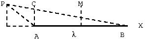
Let \(AB\) be a line charge with charge per unit length $\lambda$, which is given to be uniform. The field is to be computed at a point \(P\),. Let \(p\) be the perpendicular distance of \(P\) from the line \(AB\). let \(\alpha, \beta\) be the angles as shown in the figure. Electric field will be calculated at a general point \(P\), the corner point \(C\) and the middle point \(M\) as shown in figure below.
Let \(AB\) be a line charge with charge per unit length $\lambda$, which is given to be uniform. The field is to be computed at a point \(P\), see \Figref{LineCharge}. Let \(p\) be the perpendicular distance of \(P\) from the line \ angles as shown in the figure. Electric field is calculated at different points \(P\) as shown in figures.
 Field at a general point
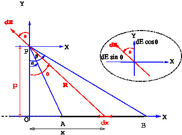
We need to choose a coordinate system. Let \(X\)- axis be taken along the line charge, the \(Y\)- axis be chosen to pass through the point \(P\).
We need to separately compute the \(x\)- and \(y\)- components of the electric field due to an element \(dx\) at position \(x\) and integrate over \(x\). The field components due to the small line element \(dx\) are\begin{eqnarray} {E}_x&=& \frac{\lambda dx}{4\pi\epsilon_0R^2}(-\sin \theta) \label{EQ01}\\
{E}_y&=&\frac{\lambda dx}{4\pi\epsilon_0R^2}(\cos\theta) \label{eq2} \end{eqnarray} The electric field is obtained by integrating over \(x\).
\begin{eqnarray} {E}_x&=&\int\frac{\lambda dx}{4\pi\epsilon_0R^2}(-\sin \theta) \label{EQ02} \\{E}_y&=&\int\frac{\lambda dx}{4\pi\epsilon_0R^2}(\cos\theta) \label{eq2a} \end{eqnarray} It is convenient to change the integration variable from \(x\) to \(\theta\) defined by $x=p \tan\theta$, and $dx=p\sec^2\theta d\theta$, with $ R=p\sec\theta$, we get \begin{eqnarray}
\nonumber {E}_x&=&\int_{\alpha}^{\beta}\frac{\lambda
p\sec^2\theta}{(4\pi\epsilon_0)p^2\sec^2\theta}(-\sin \theta)d\theta\\
\nonumber&=&\frac{\lambda}{4\pi\epsilon_0\,p}
\int_{\alpha}^{\beta}(-\sin \theta)d\theta\\
{E}_x&=&\frac{\lambda}{4\pi\epsilon_0\,p} (\cos\beta - \cos\alpha)
\label{eq3}
\end{eqnarray} Similarly, the \(y\)- component of the field works out to be
\begin{eqnarray} {E}_y&=&-\frac{\lambda}{4\pi\epsilon_0p} (\sin \beta - \sin \alpha) \label{eq4} \end{eqnarray} Thus \begin{equation} \vec E = \frac{\lambda}{4\pi\epsilon_0}\big\{(\cos\beta-\cos \alpha) \hat i + (\sin \alpha -\sin\beta) \hat j\big\} \end{equation}
Field at corner point
For a point above a corner \(\alpha=0,\beta=\pi/2\) and the field is given by
\[ E_y= - \frac{\lambda}{4\pi\epsilon_0 p} \]
Field at a point on the bisector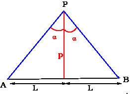
Here $\beta=-\alpha$ and $\sin \alpha=\frac{L}{\sqrt{L^2+p^2}}$ . Therefore \begin{eqnarray} {E}_y&=&\frac{\lambda }{2\pi\epsilon_0\,p}\frac{L}{\sqrt{L^2+p^2}}
\label{eq5}\\{E}_x&=&0 \label{eq6}\end{eqnarray}
Field due to an infinite line charge
In this case \(\alpha=-\pi/2. \beta=\pi/2\). Therefore the electric field at a distance \(p\) is \begin{equation} E_y = \frac{\lambda}{2\pi\epsilon_0 p}. \end{equation} This agrees with \(L\to \infty\) limit of \eqref{eq5}. In the above treatment, the field has been computed at points on the \(Y\)- axis. However, due to the rotational symmetry about the \(X\)- axis, the value of electric field will be same at all points in the \(Y-Z\) plane at a fixed distance \(\rho\) from on the \(X\)-axis.
Exclude node summary :
Exclude node links:
-

- Log in to post comments
